随机森林分类
随机森林分类
ytkz在本教程中,我们将尝试了解机器学习中最重要的算法之一:随机森林算法。我们将看看是什么让随机森林如此特别,并使用 Python 在真实世界的数据集上实现它。 您可以在此处找到代码以及数据集。
集成学习
集成方法是一种将来自多个机器学习算法的预测组合在一起以做出比任何单个模型更准确的预测的技术。由许多模型组成的模型称为集成模型。 
集成学习主要分为两类:
Boosting 和 Bootstrap
1.Boosting
Boosting 是指一组利用加权平均值将弱学习器变成更强学习器的算法。提升是关于团队合作的。每个运行的模型都决定了下一个模型将关注的功能。
顾名思义,提升意味着一个人正在向另一个人学习,这反过来又促进了学习。
2.Bootstrap
Bootstrap 是指有放回的随机抽样。Bootstrap 使我们能够更好地理解数据集中的偏差和方差。自举涉及对数据集中的一小部分数据进行随机抽样。
Bagging 是一种通用过程,可用于降低那些具有高方差的算法的方差,通常是决策树。Bagging 使每个模型独立运行,然后在最后聚合输出而不优先于任何模型。
决策树的问题
决策树对训练它们的特定数据很敏感。如果训练数据发生变化,最终的决策树可能会完全不同,反过来,预测也会不同。
决策树的训练计算成本也很高,存在很大的过度拟合风险,并且往往会找到局部最优值,因为它们在进行拆分后无法返回。
为了解决这些弱点,我们转向随机森林,它说明了将许多决策树组合成一个模型的力量。
什么是随机森林
随机森林是一种基于bagging的分类算法,它通过自助法(bootstrap)重采样技术,从原始训练样本集N中有放回地重复随机抽取n个样本生成新的训练样本集合训练决策树,然后按以上步骤生成m棵决策树组成随机森林,新数据的分类结果按分类树投票多少形成的分数而定。
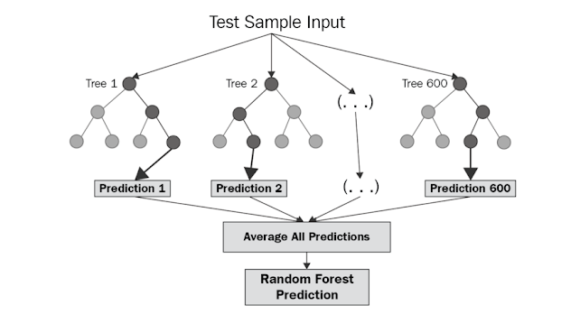
处理流程
- 从样本集中有放回随机采样选出n个样本;
- 从所有特征中随机选择k个特征,对选出的样本利用这些特征建立决策树(一般是CART,也可是别的或混合);
- 重复以上两步m次,即生成m棵决策树,形成随机森林;
- 对于新数据,经过每棵树决策,最后确认分到哪一类。
优点
- 每棵树都选择部分样本及部分特征,一定程度避免过拟合;
- 每棵树随机选择样本并随机选择特征,使得具有很好的抗噪能力,性能稳定;
- 能处理很高维度的数据,并且不用做特征选择;
- 适合并行计算;
- 实现比较简单
缺点
参数较复杂;
模型训练和预测都比较慢。
sklearn的参数
随机森林的分类学习器为RandomForestClassifier
RandomForestClassifier(
  n_estimators=10, criterion=’gini’,
  max_depth=None,min_samples_split=2,
  min_samples_leaf=1, min_weight_fraction_leaf=0.0,
  max_features=’auto’,max_leaf_nodes=None,
  min_impurity_decrease=0.0, min_impurity_split=None,
  bootstrap=True, oob_score=False, n_jobs=None,
  random_state=None, verbose=0, warm_start=False, class_weight=None)
参数解释:
控制bagging框架的参数
- estimators:随机森林中树的棵树,即要生成多少个基学习器(决策树)。
- boostrap:是否采用自助式采样生成采样集。
- obb_score:是否使用袋外数据来估计模型的有效性。
控制决策树的参数
- criterion:选择最优划分属性的准则,默认是”gini”,可选”entropy”。
- max_depth:决策树的最大深度
- max_features:随机抽取的候选划分属性集的最大特征数(属性采样)
- min_samples_split:内部节点再划分所需最小样本数。默认是2,可设置为整数或浮点型小数。
- min_samples_leaf:叶子节点最少样本数。默认是1,可设置为整数或浮点型小数。
- max_leaf_nodes:最大叶子结点数。默认是不限制。
- min_weight_fraction_leaf:叶子节点最小的样本权重和。默认是0。
- min_impurity_split:节点划分最小不纯度。
实例
from osgeo import gdal, gdal_array
import numpy as np
import matplotlib.pyplot as plt
from sklearn.ensemble import RandomForestClassifier
import pandas as pd
def main(img,lbl):
#########################################################
# Read data #
#########################################################
gdal.UseExceptions()
gdal.AllRegister()
img_ds = gdal.Open(img, gdal.GA_ReadOnly)
roi_ds = gdal.Open(lbl, gdal.GA_ReadOnly)
img = np.zeros((img_ds.RasterYSize, img_ds.RasterXSize, img_ds.RasterCount),
gdal_array.GDALTypeCodeToNumericTypeCode(img_ds.GetRasterBand(1).DataType))
for b in range(img.shape[2]):
img[:, :, b] = img_ds.GetRasterBand(b + 1).ReadAsArray()
roi = roi_ds.GetRasterBand(1).ReadAsArray().astype(np.uint8)
# 可视化
plt.subplot(121)
plt.imshow(img[:, :, 4], cmap=plt.cm.Greys_r)
plt.title('SWIR1')
plt.subplot(122)
plt.imshow(roi, cmap=plt.cm.Spectral)
plt.title('ROI Training Data')
plt.show()
# Find how many non-zero entries we have -- i.e. how many training data samples?
n_samples = (roi > 0).sum()
print('We have {n} samples'.format(n=n_samples))
# What are our classification labels?
labels = np.unique(roi[roi > 0])
print('The training data include {n} classes: {classes}'.format(n=labels.size,
classes=labels))
# We will need a "X" matrix containing our features, and a "y" array containing our labels
# These will have n_samples rows
# In other languages we would need to allocate these and them loop to fill them, but NumPy can be faster
X = img[roi > 0, :] # include 8th band, which is Fmask, for now
y = roi[roi > 0]
print('Our X matrix is sized: {sz}'.format(sz=X.shape))
print('Our y array is sized: {sz}'.format(sz=y.shape))
# Mask out clouds, cloud shadows, and snow using Fmask
clear = X[:, 7] <= 1
# 不太理解
X = X[clear, :7] # we can ditch the Fmask band now
y = y[clear]
print('After masking, our X matrix is sized: {sz}'.format(sz=X.shape))
print('After masking, our y array is sized: {sz}'.format(sz=y.shape))
#########################################################
# Random forest #
#########################################################
# Initialize our model with 500 trees
rf = RandomForestClassifier(n_estimators=500, oob_score=True)
# Fit our model to training data
rf = rf.fit(X, y)
# Setup a dataframe -- just like R
df = pd.DataFrame()
df['truth'] = y
df['predict'] = rf.predict(X)
# Cross-tabulate predictions
print(pd.crosstab(df['truth'], df['predict'], margins=True))
# Take our full image, ignore the Fmask band, and reshape into long 2d array (nrow * ncol, nband) for classification
new_shape = (img.shape[0] * img.shape[1], img.shape[2] - 1)
img_as_array = img[:, :, :7].reshape(new_shape)
print('Reshaped from {o} to {n}'.format(o=img.shape,
n=img_as_array.shape))
# Now predict for each pixel
class_prediction = rf.predict(img_as_array)
# Reshape our classification map
class_prediction = class_prediction.reshape(img[:, :, 0].shape)
# Visualize
# First setup a 5-4-3 composite
def color_stretch(image, index, minmax=(0, 10000)):
colors = image[:, :, index].astype(np.float64)
max_val = minmax[1]
min_val = minmax[0]
# Enforce maximum and minimum values
colors[colors[:, :, :] > max_val] = max_val
colors[colors[:, :, :] < min_val] = min_val
for b in range(colors.shape[2]):
colors[:, :, b] = colors[:, :, b] * 1 / (max_val - min_val)
return colors
img543 = color_stretch(img, [4, 3, 2], (0, 8000))
# See https://github.com/matplotlib/matplotlib/issues/844/
n = class_prediction.max()
# Next setup a colormap for our map
colors = dict((
(0, (0, 0, 0, 255)), # Nodata
(1, (0, 150, 0, 255)), # Forest
(2, (0, 0, 255, 255)), # Water
(3, (0, 255, 0, 255)), # Herbaceous
(4, (160, 82, 45, 255)), # Barren
(5, (255, 0, 0, 255)) # Urban
))
# Put 0 - 255 as float 0 - 1
for k in colors:
v = colors[k]
_v = [_v / 255.0 for _v in v]
colors[k] = _v
index_colors = [colors[key] if key in colors else
(255, 255, 255, 0) for key in range(1, n + 1)]
cmap = plt.matplotlib.colors.ListedColormap(index_colors, 'Classification', n)
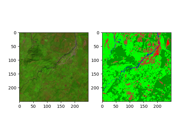
# Now show the classmap next to the image
plt.subplot(121)
plt.imshow(img543)
plt.subplot(122)
plt.imshow(class_prediction, cmap=cmap, interpolation='none')
plt.show()
a = 0
if __name__=='__main__':
img = r'LE70220491999322EDC01_stack.gtif'
lbl = r'training_data.gtif'
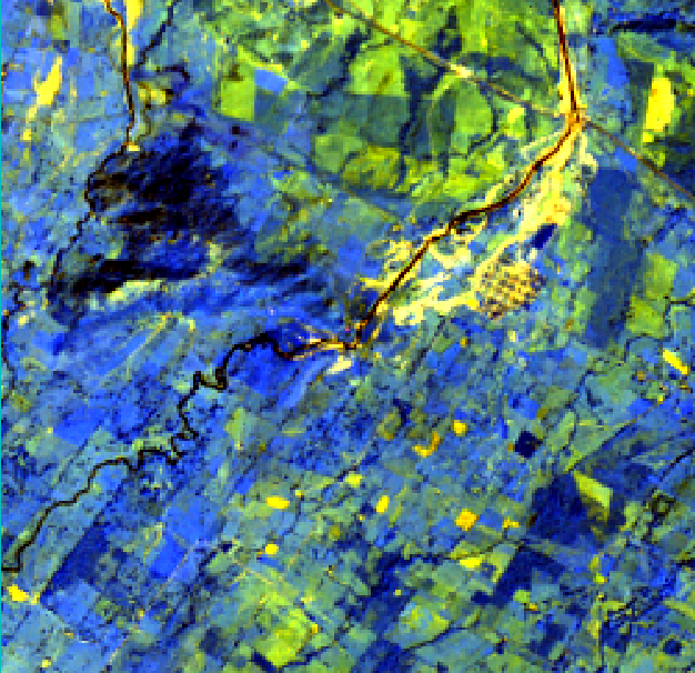
main(img,lbl)测试数据是LANDSAT 7 影像,假彩色合成如下:
百度网盘下载链接:https://pan.baidu.com/s/1-yrJpuVIr9-97aJHkvnnZA
提取码:2960