第4章-解锁地理空间分析的Python工具箱——核心工具与实战指南

第4章-解锁地理空间分析的Python工具箱——核心工具与实战指南
ytkz#
引言
地理空间分析正在成为解决全球性挑战(如气候变化、城市化、灾害管理)的关键技术,广泛应用于环境监测、城市规划、物流优化等领域。Python凭借其强大的生态系统和灵活的编程能力,已成为地理空间分析的首选语言。《Learning Geospatial Analysis with Python》(第四章“Geospatial Python Toolbox”)系统梳理了Python在地理空间领域的核心工具链,为开发者提供了从数据处理到可视化的完整解决方案。
本文将深入解析Python地理空间工具箱的核心组件,通过代码示例和实际案例,展示如何高效处理矢量、栅格和路网数据。我们还将探讨工具链的扩展、性能优化策略以及AI辅助开发的前景,帮助开发者快速构建端到端的地理空间分析工作流。
一、Python在地理空间分析中的三重角色
Python在地理空间领域的独特优势体现在以下三个层面:
- GIS脚本语言:Python提供轻量级工具(如PyShp、Fiona),用于快速操作Shapefile、GeoJSON等地理数据格式,适合原型开发和小型项目。
- 混搭粘合剂:Python无缝集成高性能C/C++库(如GDAL、GEOS),结合其简洁语法,实现高效的地理计算和数据处理。
- 全功能编程语言:Python支持构建从数据采集、处理、分析到可视化的完整工作流,适配从学术研究到企业级应用的各种场景。
代码示例:使用PyShp创建Shapefile并添加点要素
import shapefile

def create_shapefile(filename, points):
    """
    创建Shapefile并添加点要素
    参数:
        filename - 输出Shapefile路径
        points - 点数据列表 [(lon, lat, name), ...]
    """
    with shapefile.Writer(filename, shapeType=shapefile.POINT) as sf:
        sf.field("NAME", "C", size=50)  # 定义属性字段
        for lon, lat, name in points:
            sf.point(lon, lat)  # 添加点坐标
            sf.record(name)    # 添加属性值

# 示例:创建城市点Shapefile
cities = [(32.3, -90.2, "Jackson"), (30.3, -89.8, "Gulfport")]
create_shapefile("cities.shp", cities)应用:快速生成地理数据文件,适用于教学或小型GIS项目。
二、地理空间核心工具库
Python地理空间工具箱包含一系列功能强大的库,覆盖数据读写、分析、可视化和路网处理。以下是核心工具及其典型应用场景:
| 库名 | 核心功能 | 典型应用 |
|---|---|---|
| Fiona | 读写矢量数据(基于OGR) | 批量转换Shapefile为GeoJSON |
| GDAL | 栅格/矢量数据操作(格式转换、计算) | 卫星影像拼接、投影变换 |
| GeoPandas | 基于Pandas的地理数据分析框架 | 空间连接、缓冲区分析 |
| Rasterio | 简化GDAL的栅格操作API | 高程模型(DEM)处理与可视化 |
| OSMnx | 下载与分析OpenStreetMap路网数据 | 城市路网可达性分析、路径规划 |
| Folium | 基于Leaflet的交互式地图生成 | 疫情分布热力图、设施位置展示 |
| Shapely | 几何操作(空间关系、缓冲区) | 拓扑分析、几何计算 |
1. Fiona:矢量数据读写
功能:提供简洁的API读写矢量数据,支持多种格式(Shapefile、GeoJSON等)。
代码示例:将Shapefile转换为GeoJSON
import fiona
from fiona.transform import transform_geom

def convert_shp_to_geojson(input_shp, output_geojson):
    """
    将Shapefile转换为GeoJSON
    参数:
        input_shp - 输入Shapefile路径
        output_geojson - 输出GeoJSON路径
    """
    with fiona.open(input_shp, 'r') as src:
        features = []
        src_crs = src.crs
        for feat in src:
            geom = transform_geom(src_crs, 'EPSG:4326', feat['geometry'])
            features.append({'type': 'Feature', 'geometry': geom, 'properties': feat['properties']})
        geojson = {'type': 'FeatureCollection', 'features': features}

    import json
    with open(output_geojson, 'w') as f:
        json.dump(geojson, f)

# 示例
convert_shp_to_geojson("cities.shp", "cities.geojson")应用:数据格式转换,适配Web地图或跨平台共享。
2. GeoPandas:地理数据分析
功能:扩展Pandas,支持空间操作(如缓冲区、空间连接)。
代码示例:计算城市缓冲区
import geopandas as gpd

def create_city_buffers(input_shp, output_shp, buffer_distance=1000):
    """
    为城市点生成缓冲区
    参数:
        input_shp - 输入Shapefile路径
        output_shp - 输出Shapefile路径
        buffer_distance - 缓冲距离(米)
    """
    gdf = gpd.read_file(input_shp)
    utm_crs = gdf.estimate_utm_crs()  # 自动选择UTM投影
    gdf_utm = gdf.to_crs(utm_crs)
    buffers = gdf_utm.buffer(buffer_distance)
    gdf_buffers = gpd.GeoDataFrame(geometry=buffers.to_crs(gdf.crs), crs=gdf.crs)
    gdf_buffers.to_file(output_shp)

# 示例
create_city_buffers("cities.shp", "city_buffers.shp", 1000)应用:城市服务区分析、设施选址。
3. Rasterio:栅格数据处理
功能:简化GDAL的栅格操作,适合遥感影像和高程数据处理。
代码示例:计算归一化差值植被指数(NDVI)
import rasterio
import numpy as np

def calculate_ndvi(red_band_path, nir_band_path, output_path):
    """
    计算NDVI并保存为GeoTIFF
    参数:
        red_band_path - 红波段影像路径
        nir_band_path - 近红外波段影像路径
        output_path - 输出NDVI影像路径
    """
    with rasterio.open(red_band_path) as red:
        red_band = red.read(1).astype(float)
        profile = red.profile

    with rasterio.open(nir_band_path) as nir:
        nir_band = nir.read(1).astype(float)

    np.seterr(divide='ignore', invalid='ignore')  # 忽略除零警告
    ndvi = (nir_band - red_band) / (nir_band + red_band)
    ndvi = np.clip(ndvi, -1, 1)  # 标准化NDVI值

    profile.update(dtype=rasterio.float32, count=1)
    with rasterio.open(output_path, 'w', **profile) as dst:
        dst.write(ndvi, 1)

# 示例
calculate_ndvi("sentinel2_red.tif", "sentinel2_nir.tif", "ndvi.tif")应用:农业监测、植被覆盖分析。
4. Folium:交互式地图
功能:基于Leaflet生成Web交互式地图,支持标记、热力图等。
代码示例:创建城市位置地图
import folium

def create_interactive_map(center, points, output_html):
    """
    生成交互式地图
    参数:
        center - 地图中心 [lat, lon]
        points - 点数据列表 [(lat, lon, name), ...]
        output_html - 输出HTML路径
    """
    m = folium.Map(location=center, zoom_start=10, tiles="OpenStreetMap")
    for lat, lon, name in points:
        folium.Marker([lat, lon], popup=name, tooltip=name).add_to(m)
    m.save(output_html)

# 示例:密西西比州城市
center = [32.3, -90.2]
points = [(32.3, -90.2, "Jackson"), (30.3, -89.8, "Gulfport")]
create_interactive_map(center, points, "mississippi_map.html")应用:疫情分布、设施位置展示。
5. OSMnx:路网分析
功能:从OpenStreetMap下载路网数据,支持可达性分析和路径规划。
代码示例:分析城市路网
import osmnx as ox

def analyze_city_network(city_name, output_gpkg):
    """
    下载并分析城市路网
    参数:
        city_name - 城市名称
        output_gpkg - 输出GeoPackage路径
    """
    G = ox.graph_from_place(city_name, network_type="drive")
    gdf_nodes, gdf_edges = ox.graph_to_gdfs(G)
    gdf_edges.to_file(output_gpkg, layer="roads", driver="GPKG")

# 示例
analyze_city_network("Jackson, Mississippi, USA", "jackson_roads.gpkg")应用:交通规划、物流优化。
三、数据处理全流程实战
以下展示一个完整的地理空间分析工作流,涵盖数据获取、处理和可视化。
1. 数据获取与解压
场景:从在线资源下载压缩的Shapefile并解压。
代码示例:
import zipfile
import requests

def download_and_extract(url, extract_dir):
    """
    下载并解压地理数据
    参数:
        url - 数据下载链接
        extract_dir - 解压目录
    """
    response = requests.get(url)
    zip_path = "temp.zip"
    with open(zip_path, 'wb') as f:
        f.write(response.content)

    with zipfile.ZipFile(zip_path, 'r') as zip_ref:
        zip_ref.extractall(extract_dir)

# 示例:假设下载密西西比州城市数据
download_and_extract("https://example.com/MSCities_Geo_Pts.zip", "data/")注意:需确保URL有效,实际应用中可使用USGS或OpenStreetMap数据源。
2. GPS数据处理(GPX/NMEA)
GPS数据常以GPX(XML格式)或NMEA(文本格式)存储,需解析为经纬度。
代码示例:解析NMEA数据
import re

def parse_nmea_sentence(nmea_sentence):
    """
    解析NMEA GPGGA语句获取经纬度
    参数:nmea_sentence - NMEA语句
    返回:(lat, lon) 或 None
    """
    pattern = r'\$GPGGA,.*?(\d{2})(\d{2}\.\d+),([NS]),(\d{3})(\d{2}\.\d+),([EW])'
    match = re.match(pattern, nmea_sentence)
    if match:
        lat_deg, lat_min, lat_dir, lon_deg, lon_min, lon_dir = match.groups()
        lat = float(lat_deg) + float(lat_min) / 60
        lon = float(lon_deg) + float(lon_min) / 60
        if lat_dir == 'S':
            lat = -lat
        if lon_dir == 'W':
            lon = -lon
        return lat, lon
    return None

# 示例
nmea = "$GPGGA,002153.00,3342.6618,N,11751.3858,W,1,10,,33.9,M,-25.7,M,,*7F"
print(parse_nmea_sentence(nmea)) # 输出 (33.71103, -117.85643)应用:无人机轨迹分析、车辆定位。
3. 数据处理与可视化
场景:读取城市点数据,生成缓冲区并可视化。
代码示例:
import geopandas as gpd
import folium

def process_and_visualize(input_shp, output_html, buffer_distance=1000):
    """
    读取城市点,生成缓冲区并可视化
    参数:
        input_shp - 输入Shapefile路径
        output_html - 输出HTML路径
        buffer_distance - 缓冲距离(米)
    """
    gdf = gpd.read_file(input_shp)
    utm_crs = gdf.estimate_utm_crs()
    gdf_utm = gdf.to_crs(utm_crs)
    buffers = gdf_utm.buffer(buffer_distance).to_crs(gdf.crs)

    m = folium.Map(location=[gdf.geometry.y.mean(), gdf.geometry.x.mean()], zoom_start=10)
    for _, row in gdf.iterrows():
        folium.Marker([row.geometry.y, row.geometry.x], popup=row.get('NAME', 'City')).add_to(m)
    gdf_buffers = gpd.GeoDataFrame(geometry=buffers, crs=gdf.crs)
    folium.GeoJson(gdf_buffers).add_to(m)
    m.save(output_html)

# 示例
process_and_visualize("cities.shp", "city_buffers_map.html", 1000)应用:城市服务覆盖分析。
四、工具链扩展与性能优化
1. 依赖管理:Anaconda
地理空间库(如GDAL、Rasterio)依赖复杂,使用Anaconda简化安装。
命令:
conda create -n geo_env python=3.10
conda install -c conda-forge geopandas rasterio fiona folium osmnx优势:一键安装,避免编译问题。
2. 混合编程模式
场景:遥感影像处理(如NDVI计算)涉及大量数值运算,Python原生性能不足。
优化方案:
- C扩展:GDAL和Rasterio底层基于C/C++,提供高性能计算。
- Cython:将性能瓶颈部分重写为Cython,加速循环操作。
- NumPy:向量化运算,替代Python循环。
代码示例:使用Cython优化NDVI计算
# ndvi_cython.pyx
cimport numpy as np

def calculate_ndvi_cython(np.ndarray[np.float32_t, ndim=2] red, np.ndarray[np.float32_t, ndim=2] nir):
    cdef np.ndarray[np.float32_t, ndim=2] ndvi = (nir - red) / (nir + red)
    ndvi = np.clip(ndvi, -1, 1)
return ndvi编译与调用:
cythonize -i ndvi_cython.pyx
import rasterio
from ndvi_cython import calculate_ndvi_cython

with rasterio.open("sentinel2_red.tif") as red:
    red_band = red.read(1).astype(np.float32)
with rasterio.open("sentinel2_nir.tif") as nir:
    nir_band = nir.read(1).astype(np.float32)
ndvi = calculate_ndvi_cython(red_band, nir_band)优势:Cython可将性能提升10-100倍,适合大规模影像处理。
3. 并行化与分布式计算
工具:Dask-GeoPandas、joblib
场景:处理TB级遥感数据或百万级矢量要素。
代码示例:并行处理缓冲区
from joblib import Parallel, delayed
import geopandas as gpd

def parallel_buffers(gdf, buffer_distance=1000, n_jobs=-1):
    """
    并行生成缓冲区
    参数:
        gdf - GeoDataFrame
        buffer_distance - 缓冲距离(米)
        n_jobs - 并行进程数(-1表示所有CPU核心)
    """
    utm_crs = gdf.estimate_utm_crs()
    gdf_utm = gdf.to_crs(utm_crs)

    def buffer_single(geom):
        return geom.buffer(buffer_distance)

    buffers = Parallel(n_jobs=n_jobs)(
        delayed(buffer_single)(geom) for geom in gdf_utm.geometry
    )
    return gpd.GeoDataFrame(geometry=buffers, crs=utm_crs).to_crs(gdf.crs)

# 示例
gdf = gpd.read_file("cities.shp")
gdf_buffers = parallel_buffers(gdf, 1000)
gdf_buffers.to_file("parallel_buffers.shp")应用:大规模空间分析。
五、AI辅助开发
AI工具(如ChatGPT、Grok)可加速地理空间代码开发,尤其在生成原型和调试方面。
示例Prompt:
用Python读取Shapefile,计算点要素的1公里缓冲区,输出为GeoJSON。
输出(优化版):
import geopandas as gpd

def create_buffers_to_geojson(input_shp, output_geojson, buffer_distance=1000):
    """
    为点要素生成缓冲区并保存为GeoJSON
    参数:
        input_shp - 输入Shapefile路径
        output_geojson - 输出GeoJSON路径
        buffer_distance - 缓冲距离(米)
    """
    gdf = gpd.read_file(input_shp)
    utm_crs = gdf.estimate_utm_crs()
    gdf_utm = gdf.to_crs(utm_crs)
    buffers = gdf_utm.buffer(buffer_distance).to_crs(gdf.crs)
    gdf_buffers = gpd.GeoDataFrame(geometry=buffers, crs=gdf.crs)
    gdf_buffers.to_file(output_geojson, driver="GeoJSON")

# 示例
create_buffers_to_geojson("points.shp", "buffers.geojson", 1000)注意:AI生成代码需验证CRS选择和数据格式兼容性。
六、总结与资源
本文基于《Learning Geospatial Analysis with Python》第四章,系统介绍了Python地理空间工具箱的核心组件和实战应用。核心要点包括:
- 工具生态:Fiona、GeoPandas、Rasterio等覆盖矢量、栅格和可视化需求。
- 全流程支持:从数据获取(GPS、Shapefile)到处理(缓冲区、NDVI)再到可视化(Folium)。
- 优化策略:Cython、并行计算和分布式框架提升性能。
- AI助力:加速代码生成和调试。
推荐工具链组合
- 轻量级分析:GeoPandas + Folium + OSMnx,适合快速原型和Web可视化。
- 遥感处理:Rasterio + NumPy + Matplotlib,处理高分辨率影像。
- 工程化部署:PostGIS(空间数据库)+ FastAPI(API服务)+ Leaflet(前端渲染)。
学习路径
- 入门:从GeoPandas和Folium开始,掌握基本数据处理和可视化。
- 进阶:深入GDAL/Rasterio,理解栅格和矢量底层操作。
- 高级:探索Dask-GeoPandas(分布式计算)、PyVista(3D分析)和GeoAI。
推荐资源
- 文档:GeoPandas(https://geopandas.org/)、Rasterio(https://rasterio.readthedocs.io/)
- 社区:OSGeo(https://www.osgeo.org/)、StackExchange GIS
- 数据集:OpenStreetMap(https://www.openstreetmap.org/)、USGS Earth Explorer(https://earthexplorer.usgs.gov/)
结语
Python地理空间工具箱为开发者提供了从轻量脚本到工程化部署的完整解决方案。凭借Fiona、GeoPandas、Rasterio等工具的强大功能,开发者能够快速应对从城市路网分析到遥感影像处理的各种场景。结合AI辅助开发和云计算,地理空间分析正迈向智能化、实时化。掌握这些工具和技术,不仅能解决传统GIS任务,还能为智慧城市、自动驾驶等前沿领域提供支持。