3D Geospatial Data Integration with Python: The Ultimate Guide
3D Geospatial Data Integration with Python: The Ultimate Guide
ytkz3D Python
The pace of technological progress is just plain crazy nowadays. Even more so when looking at how vital 3D data is for geospatial analysis and digital twins. Being able to capture and analyze data in three dimensions means we can create precise representations of real-world objects and environments.

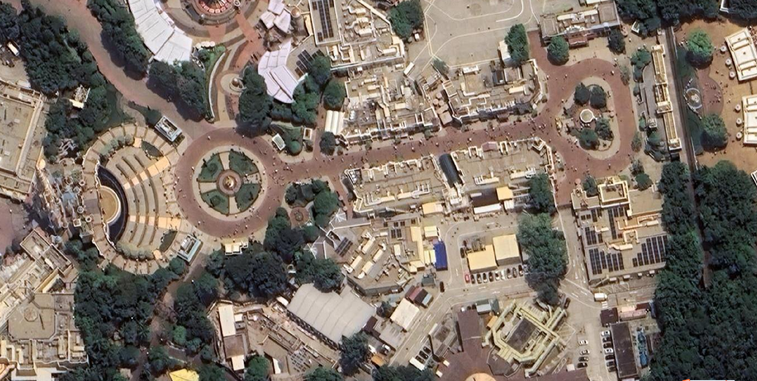
🦄Mila: A picture is worth a thousand words. So what about Digital Twins?
This is especially important for fields like urban planning, infrastructure management, and disaster response.
By incorporating 3D data, we can enhance our ability to make informed decisions by relying on precise and reliable data representations. Furthermore, the integration of this data into digital twins can produce remarkably lifelike replicas of real-world assets and systems, thereby increasing the efficiency of simulation and analysis.
BUT (there is always a but), effective geospatial analysis and digital twin creation rely on efficiently integrating and visualizing different data formats. To achieve this, it’s essential to have a comprehensive understanding of the various data modalities and how they can be seamlessly integrated and visualized together. In data terms, we want to create a unified and comprehensive representation of an area with data overlap. How lucky are we, because this is precisely what we will unlock today!

In this hands-on guide, I provide a reference system-oriented workflow for 3D data integration with Python. So no need for expensive software or a large serialized pipeline of bricks without mortar! Just our Python friend and a carefully selected tiny range of robust modules and functions.
The ultimate goal of this initiative is that you have a comprehensive guide and companion that will follow you along your 3D data journey! The workflow is structured in seven distinctive phases, as shown below.

Each phase builds progressively to ensure that you can start from scratch or plug into your existing system modularly. Because it is exhaustively constructed, a table of contents will make it easier for you to go through!
Chapter 1. 3D Python Setup1.1. Environment Setup1.2. Base Libraries1.3. 3D Data Libraries1.4. Geospatial Libraries1.5. IDE SetupChapter 2. Multi-Modal Data Curation2.1. 3D Data Sourcing2.2. Spatial Raster (GIS)2.3. Vector Data (GIS)2.4. Other SourcesChapter 3. Data Analysis and Profiling3.1. 3D Point Clouds and voxels3.2. 3D mesh and city models3.3. Spatial / Raster Imagery3.4. DSM, DTM, CHMChapter 4. Registration / Reprojection4.1. Selecting a Reference System4.2. Data Georeferencing4.3. Data Reprojection4.4. Rigid RegistrationChapter 5. Data Pre-Processing5.1. Data Cleaning5.2. Data Transformation5.3. Data Reduction5.4. Data Enrichment (Fusion)Chapter 6. Data Visualization and Validation6.1. 3D Data Inspection6.2. Point Cloud Canonical Link6.3. Hybrid Multi-Modal Visualization6.4. Projection-based InspectionChapter 7. Data Sharing7.1. Selection Method Definition7.2. Data Organization7.3. File Format Definition7.4 Export and External UseWhenever you are ready, let us jump together on this marvelous quest to 3D Data Integration, with a coffee lying around, but not too close to your computer ☕ (speaking from devastating experience)
🎵 Note to Readers: This hands-on guide is part of a UTWENTE joint work with co-authors 🦊 F. Poux*, 🦄 __M. Koeva*, and 🦝 P. Nourian**. We acknowledge the financial contribution from the digital twins @ITC -project granted by the ITC faculty of the University of Twente. All images are © F. Poux
Step 1. Implementation Setup for 3D Data

The first mission is quickly setting up a lightweight environment for developing our 3D Data Integration workflow. This is a simple phase, but ensuring a proper setup is the key to scalability and replication. So let us get on top of things!

A Lightweight Environment Setup
Python environment setup using Anaconda, robust libraries, and an Integrated Development Environment (IDE) does not have to be painful. Anaconda provides a convenient way to manage Python packages and environments, and you can then use a powerful IDE such as Jupyter Lab or Spyder to make coding a breeze. For a detailed view of the process of setting up a 3D Python development environment, I recommend that you check out the following article:
3D Python Workflows for LiDAR City Models: A Step-by-Step Guide The Ultimate Guide to unlocking a streamlined workflow for 3D City Modelling Applications. The tutorial covers Python…
🦊 Florent: If you do not want to jump on another session, do not worry, I will not leave you high and dry! As part of this ultimate guide, here is a superb lightweight setup to get started, under 5 minutes, clocked ⌚.
To start things off, you can go to the Anaconda website and download a Miniconda installer (a free minimal installer for conda) appropriate for your operating system (Windows, macOS, or Linux), with a Python 10 version. From there, you can follow the installation instructions on the Anaconda website to install Miniconda on your machine.
And that is it! You now have secured the most uncomplicated Python installation with the lightweight miniconda that will make it super easy to isolate a controlled virtual environment. Before moving on to the following steps, we launch miniconda with its command line access:

Once in the Anaconda Prompt, we follow a simple four steps process to be up and running, as shown below.

- To create a new environment, we write the line:
conda create -n GEOTUTO python=3.10 - To switch to the newly created environment, we write:
conda activate GEOTUTO - To check the Python version,
python --version, and the installed packages:conda list. This should yield Python 3.10 and the list of base libraries respectively - To install pip in the new environment, we write:
conda install pip
And that is it! We are now ready to move on installing the necessary libraries for 3D Data Integration with the pip manager: pip install package-name, where you change the package name by each of these (one at a time: numpy, matplotlib, laspy[lazrs,laszip], open3d, rasterio, geopandas.
Python base libraries

The first package installation is done via the prompt: pip install numpy.No need to present NumPy, Python’s fundamental numerical and scientific computing library. It supports large multi-dimensional matrices and provides a collection of mathematical functions to work with ease. NumPy is the foundation of many other scientific libraries in Python and is heavily used in data analysis, machine learning, and scientific research.
🦝 Nourian: NumPy is all about Linear Algebra. If you need to get comfortable with re-learning Linear Algebra, you can start from here: Rudiment of Linear Algebra for Computer Graphics (ResearchGate)
Matplotlib is a popular plotting library for Python that enables 2D plotting and basic 3D plotting capabilities. To install it: pip install matplotlib. It provides a wide range of customizable visualization options, allowing users to create various types of plots, such as line plots, scatter plots, bar plots, histograms, 3D plots, and more. Matplotlib is widely used in scientific research and data science workflows.
3D Python Libraries

Open3D is a modern 3D data processing and visualization library, mainly focusing on 3D point clouds and meshes. It provides functionalities to handle 3D data, such as point cloud registration, geometry processing, mesh creation, and visualization. Open3D is particularly useful for tasks related to 3D computer vision, robotics, and augmented reality applications. And for installing Open3D: pip install open3d.
Then, we have to install Laspy: pip install laspy[lazrs,laszip]. This Python library is used for reading, writing, and modifying LiDAR data stored in the LAS (LiDAR data Exchange Format) and LAZ (compressed LAS) file formats. It provides tools to work with point cloud data obtained from LiDAR scanners and is widely (small world) used in geospatial applications for terrain modeling, forestry, urban planning, and more.
Geospatial Libraries
Geopandas is a library built on top of pandas and shapely designed to handle geospatial data efficiently. To install it: pip install geopandas. It extends the capabilities of pandas to include geospatial data types and operations, allowing users to work with vector data (points, lines, polygons) and efficiently perform geospatial analysis. Geopandas is widely used in GIS, cartography, and spatial data analysis.
Rasterio is the last library that we will install with: pip install rasterio. It is used for reading and writing geospatial raster data. It supports various standard raster formats like GeoTIFF or JPEG and provides functionalities for geospatial metadata, spatial referencing, and coordinate transformations. rasterio is valuable for satellite imagery analysis, remote sensing, and GIS (Geographic Information Systems) applications.
Each of these libraries serves a synergic purpose and permits handling a myriad of data types in scientific computing, data science, and geospatial applications.
Setting up an IDE
The last step of our setup is to install an IDE. We are still in the command line interface within the environment, and we type: pip install jupyterlab, which will install jupyterlab on our environment. To use it clearly, we can change the directory to the parent directory of our project (let us call it INTEGRATION), which will hold both a CODE folder and a DATA Folder: cd C://COURSES/POUX/INTEGRATION. And then, we will launch jupyterlab from this location by typing in the console: jupyter lab, which will open a new localhost page in your web browser (Chrome would be the preferred choice, but Firefox or Safari work as well).
Well done! Phase one was completed successfully! 🎯We are now ready to attack the second phase: finding datasets that we can combine for later use in our NASA-graded workflow. 🙃
Step 2. Multi-Modal Data Curation

We want to integrate multi-modal datasets. But what is this swearword: multimodal? It refers to data that spans different types and contexts, such as images, point clouds, text, and sound…

🦝 Nourian: Additionally, here is a nice hitchhiker’s guide to Web-based computing platforms for Urban Planning: Essential Guide (ResearchGate)
So, our goal in this phase is to identify a zone of interest and gather as much data as possible to help us in our future analysis. The zone of interest selected today is a part of Enschede, a city in Eastern Netherlands in the province of Overijssel (Twente region), where, it makes sense, the University of Twente shines its knowledge beams. 🌞

🦄 Mila: By unlocking the secrets of our cities through the fusion of 3D geospatial and remote sensing data, we give birth to city digital twins that illuminate the past, navigate the present, and shape. If you want to dive even more into data integration on the web using open-source tools, here is a research paper: 3D Data integration for web-based opensource WebGL interactive visualization. 4/W4-2022 ed. Vol. 48. p. 89-94 6 p. (International Archives of the Photogrammetry, Remote Sensing and Spatial Information Sciences - ISPRS Archives).) (ISPRS Archives)
We are now ready to source different datasets. For clarity concerns, I organized this sourcing into four categories by searching for 3D datasets, Spatial Rasters, vector datasets, and finally from other sources, as shown below.

3D Data Sourcing
The first step is to source some datasets from some open data repository with a data license that allows us to do some experiments. On that front, for the Netherlands, there is the possibility of obtaining LiDAR data, elevation data models, and raster imagery from one place: geotiles.nl. You can zoom in on the original tiles and get access to the various datasets download links, as shown below.

🦊 Florent: To serve you best, all the used data is available in the Drive Folder shared at the end of the section. The AHN version is AHN4.
The second place you can explore to get CityModels is 3D BAG, which stands for 3D Register of Buildings and Addresses (BAG), the most detailed, openly available data set on buildings and addresses in the Netherlands. It contains 3D models at numerous levels of detail, generated by combining two open data sets: the building data from the BAG and the height data from the AHN. Using the 3D Bag Viewer by tile queries, you can explore and access the buildings.

The tile extent differs from what we got from the geotiles.nl, making it interesting when we attack the integration phase. At this stage, we already have exciting datasets under our hands. We can now move on to exploring spatial raster datasets.
Spatial Raster Data sources
For satellite and aerial imagery, the USGS Earth Explorer is one of the largest free data sources. It is worldwide, with a friendly user interface that makes accessing remote sensing data simple. It even has a bulk download application if you need to download more than one data set. If this is the first time for you, you will need to execute one additional step: creating an account, but it is free and quick (I did it in under 2 minutes ⌚).

I drew a polygon from the WebUI and then asked to get the Landsat > Landsat Collection 2 — Level 1 group (the most recent Landsat imagery is L8–9 OLI/TIRS and L7 ETM+). The differences between the collections are based on data quality and level of processing. USGS has classified images into tiers based on quality and processing level (Source). Once in the result section, you can check the footprint before deciding which would best fit your needs, as shown below.

For Digital Elevation models, I suggest sticking with the geotiles.nl data service as it is already on point with the most up-to-date and precise elevation models from the AHN. We are moving at an incredible pace, and the next stage is to get some excellent vector datasets!
Vector data curation
If you are in the GIS community, I hope presenting the power of OpenStreetMap (OSM) will not insult your knowledge base.

OSM provides different maps and layers with a crowd-sourcing initiative that makes it highly exhaustive, with a precision flag nevertheless. Indeed, OSM is open to the public and created by a general audience. So this means that accuracy can vary based on the creator and its “mapping” expertise level. However, OSM is a goldmine for openly licensed street-level GIS data.
We have several ways to download OpenStreetMap data to get our hands on some of this gold. Conveniently, there is even an OSM Data Wikipedia page with all the available OSM extracts. My recommendation is the use of the tool Geofabrik. Indeed, you can then leverage a data organization by semantic spatial extent (E.g.: country, state, continent …). You can quickly choose a geographic location and then download OSM data, as shown below.

🦊 Florent: I also prefer downloading OSM data as shapefiles, but more on that later 😉. Mila makes me think that a great piece of knowledge is distilled in this Geospatial Data with Python.
We now have some 3D datasets, some raster datasets, and vector shapefiles. Time to dig the world wide web to find other precious stones 💎.
Other sources
Well, here, the web is your ally. You can find anything you want to tie to your analyses, from web pages to news, to sounds to real-time data feeds. I would not overstate that sky (or your bandwidth 😁) is the limit! But, let me be very pragmatic again and also guide you toward one platform: Mappillary.
Mappillary is a platform that makes street-level images and map data available to scale. You can explore it and download some 360° imagery and points of interest using the Map Explorer.

You also have the ability to filter out elements by their class if you want to select only some elements of interest or to cross-validate information with OSM data, for example.
And now, the good news? To follow along the code lines that are coming, I alleviate for you the process of getting all of this data that you can find directly in this Data Drive Repository. Once you have what you need in your DATA folder, we can start a nice exploratory data analysis.
Step 3. Exploratory Data Analysis

At this stage, we have a Python code setup and a data setup, so we are ready to activate a deep focus mode with 15 minutes on clock timer ⌚. Indeed, we will now explore the various datasets we gathered with Python.

This means that, for each modality, we will go through reading, profiling, harmonizing, and categorizing its content. Often, that means dealing with library bidirectional communication. To stay concise, I took the liberty of regrouping some modalities together, as shown below.

Before loading anything, let us import all the libraries installed by writing in your notebook/script the following nine lines:
#base librariesimport numpy as npimport matplotlib.pyplot as plt#3D librariesimport open3d as o3dimport laspy as lp#geospatial librariesimport rasterio as raimport geopandas as gpd3D Point Clouds
Let us start with my protégés: 3D point clouds. They are essentially a collection of points in 3D space that represent a physical object or environment. These points are generated from various sources, including LiDAR, photogrammetry, Artificial Intelligence (yes, you read well), scanning devices, etc. The first dataset in our hands comes from the Aerial LiDAR AHN campaign in the LAZ file format. It spans from the LAS LiDAR data Exchange Format (LAS) as its compressed counterpart, widely used for storing LiDAR point cloud data. It supports 2D and 3D point data and attributes such as intensity and classification. To read the file with Python, we use the laspy library with its extensions, as follows:
#Load a las filelas = lp.read("../DATA/34FN2_13.laz")Great! we now have our file loaded in the las variable, which we can explore quickly using laspy functions to get possible attributes, the max value of the red channel, or the projection information:
print([dimension.name for dimension in las.point_format.dimensions])print(np.max(las.red))print(las.header.vlrs[2].string)This will yield the following:
['X', 'Y', 'Z', 'intensity', ‘return_number’, ‘number_of_returns’, ‘synthetic’, ‘key_point’, ‘withheld’, ‘overlap’, ‘scanner_channel’, ‘scan_direction_flag’, ‘edge_of_flight_line’, ‘classification’, ‘user_data’, ‘scan_angle’, ‘point_source_id’, ‘gps_time’, ‘red’, ‘green’, ‘blue’, ‘nir’, ‘Amplitude’, ‘Reflectance’, ‘Deviation’]255COMPD_CS["Amersfoort / RD New + NAP height",PROJCS[“Amersfoort / RD New”,GEOGCS[“Amersfoort”,DATUM[“Amersfoort”,SPHEROID[“Bessel 1841”,6377397.155,299.1528128,AUTHORITY[“EPSG”,”7004"]],AUTHORITY[“EPSG”,”6289"]],PRIMEM[“Greenwich”,0,AUTHORITY[“EPSG”,”8901"]],UNIT[“degree”,0.0174532925199433,AUTHORITY[“EPSG”,”9122"]],AUTHORITY[“EPSG”,”4289"]],PROJECTION[“Oblique_Stereographic”],PARAMETER[“latitude_of_origin”,52.1561605555556],PARAMETER[“central_meridian”,5.38763888888889],PARAMETER[“scale_factor”,0.9999079],PARAMETER[“false_easting”,155000],PARAMETER[“false_northing”,463000],UNIT[“metre”,1,AUTHORITY[“EPSG”,”9001"]],AXIS[“Easting”,EAST],AXIS[“Northing”,NORTH],AUTHORITY[“EPSG”,”28992"]],VERT_CS[“NAP height”,VERT_DATUM[“Normaal Amsterdams Peil”,2005,AUTHORITY[“EPSG”,”5109"]],UNIT[“metre”,1,AUTHORITY[“EPSG”,”9001"]],AXIS[“Gravity-related height”,UP],AUTHORITY[“EPSG”,”5709"]],AUTHORITY[“EPSG”,”7415"]]The third line gives us an interesting profile: the data is expressed in Amersfoort / RD New + NAP height reference system. We note that down for later.
🦊 Florent: As you can see, the first line gives us several attributes for later use. This is nice that, by default, we can store so much information in a semi-structured way. However, we need to sort out the relevancy of this information; usually, we default to using X,Y,Z, intensity, red, green, blue. I would call the other one’s bonuses 😁.
At this stage, we have no natural way to visualize if the data is correct; we have to transform it into our beloved numpy object, which we can after that convert to an open3d point cloud object to close the loop of switching between libraries. First, we convert some laspy object attributes to coords and colors numpy objects to hold our point cloud coordinates X,Y, Z and our point cloud colors:
coords = np.vstack((las.x, las.y, las.z))colors = np.vstack((las.red, las.green, las.blue))Then we transform our numpy object into an open3d object to visualize the point cloud. Unfortunately, no direct way from laspy exists, yet 😁.
pcd = o3d.geometry.PointCloud()pcd.points = o3d.utility.Vector3dVector(coords.transpose())pcd.colors = o3d.utility.Vector3dVector(colors.transpose()/255)o3d.visualization.draw_geometries([pcd])🦊 Florent*: This is a great exercise to see that switching libraries almost always comes down to losing some processing time between conversions and also exposes to possible memory errors. Therefore, always using a limited number of libraries is my advice when dealing with complex datasets and workflows.*

You can now visualize the full LiDAR point cloud within Python nicely, on par with professional software! Let us now load another point cloud to explore another widely used file format: .ply. The PLY format is used to store 3D mesh data along with attributes like color and normals. It is also suitable for point clouds with additional information.
With open3d, this is super simple; you can execute the following code to fill the pcd_itc variable with the point cloud, and the o3d.visualization function to draw the point cloud:
#Load a point cloud and visualizepcd_itc = o3d.io.read_point_cloud("../DATA/ITC_outdoor.ply")o3d.visualization.draw_geometries([pcd_itc])
This point cloud does not show any metadata information, which means that we will consider that it is expressed in a local reference system that will need to be registered somehow to a reference dataset.
🦊Florent: Spoiler alert! Point cloud dataset is like a special central rock, especially dealing with multiple modalities. Indeed, as I will show later, it can act as the canonical reference to then link all the other datasets to it. I warned you of the spoiler!
Time to move on 3D voxels 🧊
3D Voxels
Voxels are another type of 3D data format. Voxels are essentially 3D pixels that represent a volume of space. They are plain fun, and you can check their plain usefulness in the following case studies:
3D Python Workflows for LiDAR City Models: A Step-by-Step Guide The Ultimate Guide to unlocking a streamlined workflow for 3D City Modelling Applications. The tutorial covers Python…
How to Automate Voxel Modelling of 3D Point Cloud with Python Hands-on tutorial to turn large point clouds into 3D voxels 🧊 with Python and open3d. Unlock an automation workflow…t
🦝 Pirouz: Voxels are pretty much like LEGO models. Check out this paper about voxelization of spatial data and getting serious with digital LEGO: Voxelization Algorithms for Geospatial Applications (ResearchGate). If you can’t get enough of voxels? Then search Google for “voxel art” and check out the library topoGenesis (GitHub).
Now, we will read and visualize the voxel dataset with the following code lines:
vox_read = o3d.io.read_voxel_grid("../DATA/34FN2_13_vox.ply", format='auto')o3d.visualization.draw_geometries([vox_read])
At this stage, we read, profiled, and made sure that we had a way to deal with all this data with a single library for processing (numpy) and one for 3D visualization (open3d).
Time to get city models in our Python experiments 😁
City Models
Models of Cities often follow a standard of expression: CityGML models. CityGML is an XML-based data format used to represent the 3D geometry of urban environments. CityGML models can include information about buildings, roads, bridges, and other infrastructure. City planners, architects, and engineers often use these models to simulate and analyze urban environments. An excellent place to get yours, which I did not mention on purpose before, is this GitHub repository curated by my colleague Olaf (Any Frozen reference forbidden ⛄): CityGML Models.
🦊 Florent: Basically, in Python, we have to make sure to convert these models to 3D meshes while keeping any wanted semantic / topology or other information. A friendly Python tool, again by TUM, is available here: citygml2obj. But I did the heavy lifting for you if you use the data, thus moving on to the next reading modality: 3D meshes.
3D Mesh
Next, let’s talk about meshes. Triangular meshes are constituted of vertices, edges that bind vertices, and triangular faces that finish the “envelope” of objects. They allow us to depict the shape of a 3D object. Meshes can be created using 3D modeling software or generated from point clouds, city models using specialized algorithms, or even Artificial Intelligence! The dataset is in an OBJ format commonly used to export 3D mesh models representing geometry and texture coordinates.
🦝 Pirouz: If you want to know why these fancy words are used instead of points, lines, and polygons, you need to learn a bit more about another fancy word: ***topology***.
🦊 Florent: You can read a story about topology written by Pirouz which may well be one of the easiest story about topology: Rudiments of Geometry and Topology (ResearchGate)
To load the mesh and get its extent, we will write the following lines:
mesh = o3d.io.read_triangle_mesh("../DATA/10–976–660-LoD22–3D.obj")mesh.get_axis_aligned_bounding_box()And we see from the output that we have coordinates that span closely to what Amersfoort / RD New gives. This is comforting; we now have another dataset in this reference system.
From there, to visualize the mesh, we first compute some vertex normals and use the same visualization function from open3d to visualize it:
mesh.compute_vertex_normals()o3d.visualization.draw_geometries([mesh])On the 3D side, we are good to go! Let us explore our Spatial Rasters with Python and rasterio
Spatial Imagery
Our imagery is in the GeoTIFF format, an extension of the TIFF format that includes geospatial metadata, making it ideal for raster elevation data (DSM/DTM) and imagery. To open and profile the spatial imagery that we have, we simply use the following lines of code using rasterio:
sat_image = ra.open("../DATA/RGB_34FN2.tiff")sat_image_array = sat_image.read(1)print(sat_image.meta)This results in the following output:
{‘driver’: ‘GTiff’, ‘dtype’: ‘uint8’, ‘nodata’: None, ‘width’: 20002, ‘height’: 25002, ‘count’: 3, ‘crs’: CRS.from_epsg(28992), ‘transform’: Affine(0.25, 0.0, 254999.75, 0.0, -0.25, 475000.25)}Interestingly, we get a clear detail that it is an image of 20002x25002, with three channels (R,G, and B) expressed in the CRS 28992, which corresponds to Amersfoort again! This is great!
Now, to plot with numpy and matplotlib, below is the tiniest possible line of code to get an image with numpy, avoiding Memory errors, with a result shown afterward:
plt.imshow(sat_image_array)plt.axis("off")plt.show()In parallel, rasterio also provides show() function to perform everyday tasks such as displaying multi-band images as RGB and labeling the axes with proper geo-referenced extents. This permits to simplify the plot, as expressed below:
from rasterio.plot import showcir_image = ra.open("../DATA/CIR_34FN2.tiff")show(cir_image)show(sat_image)


This is superb! We have several 3D datasets (3D point clouds, voxels, 3D meshes) and satellite imagery (both infrared and R, G,B) that we could both handle with numpy and express for most of them in one common CRS. Let us move to other rasters focusing on elevation data (2.5D).
Elevation Rasters (DSM, DTM)
Elevation models are usually found as raster files, where each pixel has a value that can be translated to its elevation. This is why we call that 2.5D data as it is a pure top-down or single point of view, also tagged depth image when out of any GIS projection system. We can import elevation models with the same code line:
dtm = ra.open("../DATA/DTM5_34FN2.TIF")Now that we have a dtm variable that holds the elevation data, we extract its metadata on the whole with dtm.meta, or more specialized with dtm.shape, dtm.crs, dtm.bounds, dtm.overviews(1):
print(dtm.meta)print(dtm.shape, dtm.crs, dtm.bounds, dtm.overviews(1))This brings us to the following result:
{‘driver’: ‘GTiff’, ‘dtype’: ‘float32’, ‘nodata’: 3.4028234663852886e+38, ‘width’: 1000, ‘height’: 1250, ‘count’: 1, ‘crs’: CRS.from_epsg(28992), ‘transform’: Affine(5.0, 0.0, 255000.0, 0.0, -5.0, 475000.0)}(1250, 1000) EPSG:28992 BoundingBox(left=255000.0, bottom=468750.0, right=260000.0, top=475000.0)And again, it is interesting to see that we have the same CRS Amersfoort / RD New for this dataset.
To get a plot and a sense of what we are dealing with, we can transform the dataset to a numpy array and use indexing to select part of it in a selection variable:
dtm_array = dtm.read(1).astype(‘float64’)selection = dtm_array[300:800,300:800]Finally, we plot using the two ways: rasterio and matplotlib both the full-scale dataset and the zoomed-in selection:
#For the dtm plot with rasterioshow(dtm)#For the dtm zoomed-in plot with matplotlibfig, ax = plt.subplots(1, figsize=(15, 15))ra.plot.show(selection, cmap=’Greys_r’, ax=ax)plt.axis(‘off’)plt.show()

Finally, we cannot discuss raster datasets without diving into vector spatial data.
Spatial Vector Data
At this stage, it is essential to clarify once and for all that, if you find pixels, you are not speaking about vector data. Instead, vector datasets are made of vertices and paths, which are available as points (X, Y coordinates), lines (they connect these points now tagged vertices), and polygons (connect vertices to close a path made of lines).

🌱 Growing: Having that in mind, where does your intuition place 3D point clouds? Voxel models? 3D meshes? These are interesting questions with profound implications, but nice to situate better how 2D stands with a 3D synergy.
Interestingly, cartographers (but not only) use these as “symbols” to depict real-world components in maps. This means that they constantly have to determine a “Level of Detail” (LoD) that the entity represents, and this gives so much symbolic power to these entities (a point can be a country, or a town, or a citizen, or a specific place, …).
To handle these vector datasets, we mainly use one open specification, the shapefile format. This permits us to spatially describe geometries and attach some kind of additional information to them. On our computer, the shapefile file format is simply a collection of several files formatted to represent different aspects of geodata (Reference):
.shp— The shape file, which contains the feature geometry itself..shx—The shape index format, which holds a positional index of the feature geometry. This is very useful for large files in order to allow quick search thanks to clever “indexing”..dbf— The attribute format, which holds various attributes for each shape in a tabular way (dBase IV format).
On top, we may have optional files that accompany the shapefile format. The most noteworthy one is the “.prj“ file. This extra file actually defines the coordinate system and any projection information deemed necessary. Thus, having all these files allows us to load street data of the region Overijssel using this time geopandas:
vector_data = gpd.read_file("../DATA/gis_osm_roads_free_1.shp")
Let us now explore a bit its projection system by exploring its CRS:
print(vector_data.crs)Which results in the following:
<Geographic 2D CRS: EPSG:4326>Name: WGS 84Axis Info [ellipsoidal]:- Lat[north]: Geodetic latitude (degree)- Lon[east]: Geodetic longitude (degree)Area of Use:- name: World.- bounds: (-180.0, -90.0, 180.0, 90.0)Datum: World Geodetic System 1984 ensemble- Ellipsoid: WGS 84- Prime Meridian: GreenwichAs we can see, this dataset is expressed in the ESPG 4326, which stands for WGS84. So this is different from our other datasets so far.
Florent: geopandas is a perfect mashup of pandas and shapely. Thus if you are familiar with both, geopandas will be a breeze! Some useful commands are vector_data.columns or vector_data.describe() that can give you an overview of its content quickly.
But let us now explore our dataset visually to see its content:
vector_data.plot()Which results in the following plot:

This is very interesting! We can also use Matplotlib to display vector data. And the region is densely populated with an extensive road network, which is very dense! Let us now extract some points of interest from another source of data.
Vector: Points of Interest
The dataset pack has a GeoJSON file, a lightweight and popular format for representing vector data with geometry and attributes, suitable for web-based applications and data exchange. To load the file, we also use geopandas with this code line:
trashcan_data = gpd.read_file("../DATA/mapillary-trashcan_points.json")We profile its CRS:
trashcan_data.crsThis gives us an answer that this is in the WGS84 CRS again. Finally, we plot to check any abnormality firsthand:
trashcan_data.plot()
This may be a bit bland without any more context; thus, layering Raster imagery would be a first choice already. But before that, let us explore another dataset we could try: 360° imagery!
360° Imagery
From the mappillary platform, we have the ability to extract some 360° images that come with a specific license to be used. You can still use geopandas to read these images :
image = ra.open("../DATA/An8XJdYJkSXycbyDWiVyw8dfVi2IzZ-jr9z7IxneeEXnOJPt0K1C89cMdXNkl5FZT0x6aVuPFRpda6eWV9fcnpgJkPfWjrd7k9harUP48csXGFf2azE1qF7FhkYK4h__j9t6Vd3aUfKcEdlqF_rsVO4.jpg")print(image.meta)That will output:
Dataset has no geotransform, gcps, or rpcs. The identity matrix will be returned. dataset = DatasetReader(path, driver=driver, sharing=sharing, **kwargs){'driver': 'JPEG', 'dtype': 'uint8', 'nodata': None, 'width': 2048, 'height': 1024, 'count': 3, 'crs': None, 'transform': Affine(1.0, 0.0, 0.0, 0.0, 1.0, 0.0)}Here we can see (of course) that this image has no geotransform data. And this is normal: this is not a spatial raster! However, if we wanted, we could add a position so that a data point represents the place the picture was taken, a hint at layering data modalities through data integration. But before going there, let us plot the image:
ra.plot.show(image)This results in the following:

We have now successfully loaded 3D Point Clouds, 3D City models as 3D Meshes, 3D Voxel dataset, Spatial rasters (satellite imagery, aerial imagery, and elevation rasters), vector datasets (lines and points), as well as 360° imagery. The first objective is now an evident success! But, we need to check how to bring that all together, and the first thing to check is actually if they are expressed in the same Coordinate Reference System (CRS). For that, I compiled the results of our profiling step in the table below.
| Data | Lidar Point Cloud | TLS Point Cloud | 3D City Mesh | Satellite Imagery | Digital Terrain Model | Streets (Vector) | Trashcans ||------|----------------------------------|-----------------|----------------------------------|---------------------|-----------------------|--------------------------|--------------------------------|| Name | 34FN2_13.laz | ITC_outdoor.ply | 10-976-660-LoD22-3D.obj | RGB_34FN2.tiff | DTM5_34FN2.TIF | gis_osm_roads_free_1.shp | mapillary-trashcan_points.json || CRS | Amersfoort / RD New + NAP height | None | Amersfoort / RD New + NAP height | Amersfoort / RD New | Amersfoort / RD New | WGS 84 | WGS 84 || CRSC | 7415 | | 7415 | 28992 | 28992 | 4326 | 4326 |We see a mix of EPSG:7415, 28992, 4326 or missing EPSG. The next stage is thus to clarify and use a unifying system for all datasets.
Data Registration and Reprojection

Before integration, we have to ensure that all datasets are in a compatible format and coordinate reference system (CRS). If this is not the case, we perform data reprojection to bring them into a common CRS. This is achieved in four main stages by (1) Selecting a reference system, (2) Georeferencing the primary dataset, (3) Reprojecting other datasets, and (4) Aligning rigidly local datasets, as shown below.

Let us go through these stages.
Selecting a Reference System
Alright, let us dive into the exciting world of reference systems! Imagine reference systems as the GPS coordinates that guide your data through the vast landscape of planet Earth. A reference system defines a set of rules and parameters to represent the Earth’s surface in a way that makes sense to us mere mortals. It’s like choosing a secret language that your data speaks fluently, allowing it to find its place in the world. Now, how do we choose the correct reference system? Let’s be pragmatic and attempt to first delineate the scope + region of interest of the project at hands.

Different reference systems work better for different parts of the globe. Something like the Amersfoort / RD New can be a fantastic choice for local projects in the Netherlands. The trusty WGS84 or Universal Transverse Mercator (UTM) might be your best buddy for more global ventures. Therefore, we use the Amersfoort / RD New + NAP height (for the elevation information) as our CRS.
Remember, when choosing a reference system, let the nature of your project and the region guide your decision. Pick a system that speaks the language of your data and brings harmony to your geospatial endeavors.🗺️
Data Georeferencing
Okay, we have our CRS defined; this step ensures that the data tagged in EPSG:7415 for 3D data, and EPSG:28992 for 2D data. When profiling, we could then check that these datasets are already coherent:
- LiDAR 3D Point Cloud
- Raster Imagery (both Spatial Raster and Elevation Raster)
However, the voxel dataset and the mesh from the city model dataset look like they are in the same CRS but have no metadata. Thus, we quickly overlay these datasets to check for any possible inconsistencies:
o3d.visualization.draw_geometries([pcd,vox_read,mesh])Which results in the following:

🦊Florent: Everything is aligned nicely, as shown in the image. The various datasets are cut on purpose to show the overlap between them. You can also see that point clouds have a bit more roughness and “resolution” over the 3D models that represent the buildings.
the remaining datasets to address are the following:
- Vector datasets (both the OSM and Mappillary one) that are expressed in WGS84
- The ITC Point Cloud dataset is not georeferenced.
Let us then deal with data projection first.
Data Reprojection
Spatial data reprojection is a fundamental process that involves transforming spatial data from one coordinate reference system to another, typically to match the projection and coordinate units of a specific spatial analysis. Reprojection ensures that different datasets with distinct projections can be accurately overlaid, integrated, or analyzed.
The process involves mathematical calculations that convert geographic coordinates (latitude and longitude) from one datum to another, considering parameters like scale, rotation, and distortion. Spatial data reprojection is essential for achieving data consistency, enabling interoperability between different datasets, and conducting accurate geospatial analyses across diverse mapping systems and applications.
When reprojecting spatial data between reference systems, several important factors must be carefully considered to ensure accurate and meaningful results. Here are some of the key considerations:
- Coordinate Systems and Projections: Understand the coordinate systems and projections of both the source and target reference systems. Make sure they are compatible; if not, choose an appropriate transformation method.
- Datum and Ellipsoid: Check the datums and ellipsoids used in the source and target systems. Differences in datums can lead to significant shifts in coordinates. Apply datum transformations if needed to align the data correctly. If you feel a bit confused, here is a nice lecture on datum and ellipsoid (tamia.edu)
- Accuracy / Precision: While these pinpoint two different characteristics (which extends the scope of our article), it is important to understand the required “level” for your specific analysis. Reprojection can introduce some errors, especially in large-scale transformations. Indeed, any data “error” has a potential impact on the results of our analysis.
- Distortions: Different map projections can introduce distortions in shape, area, distance, or angles. Be aware of these distortions and their implications on your data interpretation.
- Coverage Area: Some projections are suitable for specific regions but may not be ideal for global datasets. Choose a projection that preserves the properties of your data over the entire coverage area.
- Metadata and Documentation: Keep track of the reprojection process and document the transformations applied to the data. Properly document the source coordinate system and the target projection for future reference.
By carefully considering these factors, we ensure that reprojection is performed accurately and the resulting data is suitable for our intended applications. It is essential to be mindful of potential errors and artifacts that can arise during the reprojection process and to validate the results to maintain the quality and reliability of the data. In our case, we have to reproject both vector datasets. To do this, we use the following lines:
trashcan_data_georeferenced = trashcan_data.to_crs(‘epsg:28992’)trashcan_data_georeferenced.plot(color=’red’)vector_data_georeferenced = vector_data.to_crs(‘epsg:28992’)vector_data_georeferenced.plot(edgecolor=’green’)Which results in the following:


🦊 Florent: 3D Reprojection is also possible, but currently extend a bit the scope of this guide. Nevertheless, you can browse the library of course tutorials, where you will find some nice code and examples for 3D reprojection in the context of Segment Anything for Semantic Segmentation.
Note the change in the coordinates on the axes of our plots! At this stage, it looks like we only have one data to register: the 3D Point Cloud of ITC.
Data Rigid Registration

In 3D integration, data registration becomes crucial. Point cloud registration methods are usually made of two stages: a coarse alignment to position relatively closely two point clouds quickly. Then a fine registration like Iterative Closest Point (ICP) or feature-based registration to align multiple point clouds with a higher degree of precision. To give you a hint concerning global registration, we can align the ITC point cloud by picking a list of three pairs of common points to get a first estimate, which is later refined with ICP. This permits obtaining an overlaid point cloud. These largely extend the scope of the current guide, and will be covered in another session.😉
We now possess an aligned dataset expressed in a coherent CRS. The next stage is to see if we can refine the “data oil” to get some intelligent analytical workflow that can be built from there.
Step 5. Data Processing, Transformations, and Fusion

This stage can also be done before the registration and reprojection part. Indeed, as we predominantly work per dataset, this is a solution and can impact (for better or worse) the results of the previous steps.
Spatial data integration combines different types of spatial data (2D, 3D, or 2.5D) to create a unified and comprehensive representation of an area with data overlap. This process allows us to leverage the strengths of each data type and derive more valuable insights from the integrated dataset. Here is a quick view of some processing strategies for spatial data integration:

Now, let us explore what these four main stages actually look like, code-wise.
Data Cleaning (Raster Dataset)
the first stage is to handle missing or erroneous data points carefully. Data cleaning techniques like interpolation or extrapolation may be used to fill in gaps or replace erroneous values. In our case, we could fill empty raster values from our DTM.
I do this by interpolating neighboring pixels for each empty zone to try and give a better structure to our dataset with the following code snippet:
#We import a specific functionfrom rasterio.fill import fillnodata#We transform to a numpy arraydtm_array = dtm.read(1)#We interpolateinterpolated_dtm = fillnodata(dtm_array, mask=dtm.read_masks(1), max_search_distance=100, smoothing_iterations=0)#We plot the resultsfig, ax = plt.subplots(1, figsize=(15, 15))ra.plot.show(interpolated_dtm, cmap='Greys_r', ax=ax)plt.axis('off')plt.show()🌱 Growing: How would you use this to extract contour lines on your zone?
This results in the following:

Data Transformation (3D Point Cloud)
Aside from conversion between file formats, data transformation refers to the various processes to ensure structural and content integrity toward one or more processing steps. For example, it is imperative in many feature engineering tasks to enhance 3D machine learning model performances.
One critical data transformation method is scaling, ensuring that all the values in a dataset are within a specific range, such as 0 to 1. To do this on a point cloud, we proceed as follows:
#We compute a MinMaxScaler boundscoords_itc = np.array(pcd_itc.points)min_itc = np.min(coords_itc, axis=0)max_itc = np.max(coords_itc, axis=0)#MinMaxScalingcoords_itc_mmscaling = (coords_itc - min_itc) / (max_itc - min_itc)This transforms our original point cloud with coordinates between 0 and 1 for all our points. Therefore, if we were to plot their distribution along the three axes, we would use the following:
n_bins = 20fig, ax = plt.subplots(1, 3, sharey=True, tight_layout=True)ax[0].hist(coords_itc_mmscaling[:,0], bins=n_bins, color = "skyblue")ax[1].hist(coords_itc_mmscaling[:,1], bins=n_bins, color = "salmon")ax[2].hist(coords_itc_mmscaling[:,2], bins=n_bins,color = "purple")To obtain:

As you can see, our point cloud now has X, Y, and Z coordinates that range between 0 and 1.
🍇 Note: This is interesting on another flavor. Indeed, we tend to a pattern looking at the Z distribution, where a hint toward a Z-driven algorithm makes sense, for example, to distinguish roofs from the ground points.
Data Reduction: Cropping mask, Point Cloud Sampling
Data reduction encompasses the various techniques in which data is reduced to its simplest possible form to enable optimal analytical tasks.
One of these is data cropping: reducing the spatial extent of our dataset. A clear example could be executed on raster datasets to limit the memory footprint by loading a huge zone when we want to focus on a tighter area. To do this, with rasterio, we have first to create a geopandas bounding box that will act as the filtering mask:
from shapely.geometry import PolygonBBlidar=[np.min(coords, axis=1),np.max(coords, axis=1)]minx=BBlidar[0][0]miny=BBlidar[0][1]maxx=BBlidar[1][0]maxy=BBlidar[1][1]areabbox = gpd.GeoDataFrame({'geometry':Polygon([(minx,maxy),(maxx,maxy),(maxx,miny),(minx,miny),(minx,maxy)])},index=[0],crs="EPSG:28992")We then get a nice area box that we use as a mask on the original file (or any raster of choice) by also making sure we copy the metadata of the original file onto the cropped version:
from rasterio.mask import maskin_raster = ra.open("../DATA/CIR_34FN2.tiff")# Do the clip operationout_raster, out_transform = mask(in_raster, areabbox.geometry, filled=False, crop=True)# Copy the metadata from the source and update the new clipped layerout_meta=in_raster.meta.copy()out_meta.update({ "driver":"GTiff", "height":out_raster.shape[1], # height starts with shape[1] "width":out_raster.shape[2], # width starts with shape[2] "transform":out_transform})# Plot the CIR rasterra.plot.show(out_raster)This results in the following:

Another clear data reduction technique is data sampling. In our case, trying to reduce the number of points in our point cloud. This can be done in several ways (which, again, extend the scope of this article), with one using the voxel data structure a priori: we want to keep one best candidate per voxel:
voxel_size = 1pcd_downsampled = pcd.voxel_down_sample(voxel_size = voxel_size)o3d.visualization.draw_geometries([pcd_downsampled])This results in the following downsampled point cloud:

Finally, we can enrich our dataset in various ways.
Data Enrichment: Inject POI proximity to point clouds
Depending on the application, various fusion techniques can be applied to merge the datasets. For 2D and 2.5D integration, raster-based methods like weighted averaging or majority voting can combine multiple data layers. In 3D integration, point cloud fusion techniques, such as merging, averaging, or voxelization, are employed to create a single, consolidated 3D point cloud representing the entire area.
🦊 Florent: Using data enrichment (fusion) techniques, we combine information from multiple sources (it can be web-based, from a data acquisition mission, or any relevant way to gather data). This allows the creation of a more comprehensive and accurate representation of the underlying phenomenon. These can touch on raster Weighted Averaging (Involves taking a weighted average of pixel values from multiple raster layers, where the weights represent the importance or reliability of each raster layer), Majority Voting (Combines categorical raster data by assigning the majority class to each pixel location, helpful in land cover classification). But these are for another time. 😉
A swift way to extend our dataset is to compute additional features. This is done, for example, on the 3D point clouds by extracting normals computed from a neighborhood of points that permits extracting the best fitting plane, then the normals. We automatically do this with the following piece of code:
nn_distance = np.mean(pcd.compute_nearest_neighbor_distance())print(nn_distance)#setting the radius search to compute normalsradius_normals=nn_distance*4pcd_downsampled.estimate_normals(search_param=o3d.geometry.KDTreeSearchParamHybrid(radius=radius_normals, max_nn=16), fast_normal_computation=True)# Visualizing the point cloudpcd_downsampled.paint_uniform_color([0.6, 0.6, 0.6])o3d.visualization.draw_geometries([pcd_downsampled])And as you can see below, we can visualize our new point cloud without or with normals (pressing “n“ in the interactive window viewer):


Step 6. Multi-modal Data Visualization

Multi-modal data visualization is a powerful approach that seamlessly integrates our diverse geospatial data, including vector data, spatial raster imagery, Digital Surface Models (DSM), Digital Terrain Models (DTM), point clouds, and city models.

This comprehensive fusion of data types allows for a more holistic understanding of the environment, laying the groundwork for more informed decision-making and sophisticated analyses. Now, let’s dive into a Python solution that showcases how to achieve this remarkable visualization feat!
The trick is to understand the strengths and limits of each of our libraries! Indeed, what we will do is actually to stick to Open3D to check for the consistency between the data modalities (Meshes, 3D Point Clouds, and Voxels) and use the point cloud dataset as the canonical reference to then link all the other datasets to it.

Therefore, the first step is to analyze the 3D modalities:
o3d.visualization.draw_geometries([pcd,vox_read,mesh])
🦊 Florent: While the image may be confusing, be warned that nothing is going wrong when you visualize these three in one image. Indeed, the extent of the datasets are different to allow us to delineate the modalities better visually.
Great! From there, we use the point cloud dataset with Numpy on a top-down view to check the X-Y consistency, for example, with vector data:
# Plot the Georeferenced Shapefile and Point Cloud together using matplotlibvector_data_clipped_pc = vector_data_georeferenced.cx[257000:258000, 471200:472400]fig, ax = plt.subplots(figsize=(15, 15))vector_data_clipped_pc.plot(ax=ax, color='yellow', edgecolor='yellow')# Plot the point cloudax.scatter(coords[0][::100], coords[1][::100], c=coords[2][::100])# Customize the plot (add labels, titles, legends, etc. if needed)ax.set_xlabel('X (meters)')ax.set_ylabel('Y (meters)')ax.set_title('Shapefile and Point Cloud Visualization')# Show the plotplt.show()This lays an obvious overlay of the vector dataset onto our point cloud that opens up a world of possibility to make these two dataset talk:

Then, we continue our linkage by linking the vector dataset, reprojected, with spatial imagery:
#Clipping vector datavector_data_clipped = vector_data_georeferenced.cx[255000:260000, 469000:475000]#Plot the Raster Imagery with Vector Datasetfig, ax = plt.subplots(figsize=(15, 15))ra.plot.show(sat_image, ax=ax)vector_data_clipped.plot(ax=ax, facecolor='none', edgecolor='green')#Zooming-infig, ax = plt.subplots(figsize=(15, 15))plt.axis([258000, 258500, 471000, 471500])#The line above actually define the extent of the plot using the coordinates in the CRS.ra.plot.show(sat_image, ax=ax)vector_data_clipped.plot(ax=ax, facecolor='none', edgecolor='cyan')This results in the visualization, which demands a bit of zoom, as expressed in the code, to better situate the fit of both datasets.


The exact process is repeated for the locations from Mappillary, with the code below.
#Overlaying Raster with Vector datafig, ax = plt.subplots(figsize=(15, 15))plt.axis([257600, 260000, 471000, 471500])ra.plot.show(sat_image, ax=ax)trashcan_data_georeferenced.plot(ax=ax, facecolor='none', edgecolor='green')
And finally, we want to overlay raster, vector, and point cloud modalities in one plot with Numpy:
# Plot the Shapefile and Point Cloud together using matplotlibvector_data_clipped_pc = vector_data_georeferenced.cx[257000:258000, 471200:472400]fig, ax = plt.subplots(figsize=(15, 15))# plot the sattelite imageryra.plot.show(sat_image, ax=ax)# Plot the shapefilevector_data_clipped_pc.plot(ax=ax, color='blue', edgecolor='blue')# Plot the point cloudax.scatter(coords[0][::100], coords[1][::100], c=coords[2][::100])# Customize the plot (add labels, titles, legends, etc. if needed)ax.set_xlabel('X (meters)')ax.set_ylabel('Y (meters)')ax.set_title('Shapefile and Point Cloud Visualization')# Show the plotplt.show()This little piece of code (careful on the shortcuts and smart tricks employed to condense the snippet) permits us to put a final note on the data integration of our various modalities.

We approach the end of our systematic approach!
By carefully applying these processing techniques, spatial data integration enables us to create a holistic representation of the environment, facilitating better decision-making and insights in a wide range of applications. Still, we must consider the last step: sharing the newly processed data.
Step 7. Data Sharing

Spatial data export is vital in the geospatial data workflow, allowing us to seamlessly share, visualize, and analyze 2D and 3D data modalities in established software. To this end, we can take a higher, almost aerial view to better situate the extent of data sharing impacts. I chose to relate to academia and publishing proofs of new scientific discoveries. Indeed, this process that I illustrate below is the key to an ethical and robust R&D cycle. As you can see, data export in standard formats, which we cover here, is the central link to data browsing before pushing automated solutions.

Thus, the export process must create various file formats suitable for applications and software environments. Each file format has its specificities, catering to different use cases and previously expressed requirements. For in-depth 3D data export, I propose to relate to these articles:
3D Python Workflows for LiDAR City Models: A Step-by-Step Guide The Ultimate Guide to unlocking a streamlined workflow for 3D City Modelling Applications. The tutorial covers Python…
Understanding how we can do the same with vector and raster datasets is essential. As always, the simpler, the better: let us focus on these last exporting steps. To export the raster imagery, you can do the following with rasterio:
with ra.open("../RESULTS/CIR_34FN2_cropped.tiff",'w',**out_meta) as wf: wf.write(out_raster)And concerning vector datasets, geopandas makes it a breeze to export the georeferenced and clipped result from our processing stages:
vector_data_clipped_pc.to_file("../RESULTS/roads.shp")Finally, you can import these in a software such as QGIS or CloudCompare, which results in the following:

This is the perfect layering of 3D, Raster, and Vector datasets!
Conclusion
We have embarked on an exciting journey exploring the world of 3D data integration with Python. Throughout this comprehensive guide, we have uncovered the immense potential of combining various 3D data modalities, such as point clouds, meshes, city models, DSM, DTM, and voxels, to create a unified and holistic representation of the spatial environment.
To summarize, I list below the key takeaways related to the seven steps that we covered:
- Setting up a multi-modal coding environment in Python needs to accommodate a minimal number of robust libraries.
- When sourcing datasets, it is best to carefully consider available open datasets with clear licensing options through web interfaces that make it easy for you to gather relevant samples.
- It is an excellent practice to independently profile each modality and assess its main characteristics (CRS, precision, resolution, …) through quick analysis schemes.
- Mastering Coordinate Reference Systems and knowing how to go from one another and what a specific transformation implies is mandatory for scalable workflows with spatial datasets.
- Pre-processing algorithms and techniques are often the keys between optimized and organized data assemblies and data warehouses with chaotic management systems.
- nD data visualization is paramount to a successful data integration workflow and demands that you carefully consider which dataset/ data modality acts as your canonical anchor
- Data Sharing as a final stage permits ensuring a system from A to Z that considers practical and operational considerations, even in academia or R&D actions where production phases can be overlooked.

As I conclude this guide, I cannot help but be thrilled about the future of 3D data processing. Currently, with Python’s versatility and the growing landscape of geospatial technologies, we have a large opening for new ways to better understand complex spatial phenomena (and act on them).
Therefore, you can expect an even deeper guide to efficient algorithms, innovative visualization techniques, and seamless integration with cutting-edge technologies. By exploring what we can accomplish with integrated 3D data workflows, we pave the way for new applications, some of which coming soon to your laps. This makes me say that you are on a good track to shape the future of spatial analysis and visualization, transforming how we perceive and interact with the world around us.